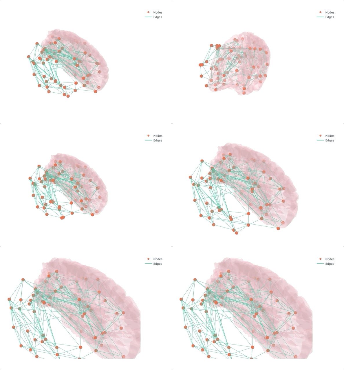
Connect, Rotate, Zoom - Interactive brain networks

If you don’t make it interactive, enjoy only half
I spent already a few posts on the topic of making ordinary stuff interactive, and despite the chances of literally wooing people when they see the final results, I think the final result is not the biggest selling point of interactive visualization. I think that what really makes interactive visualization great is the fact that makes it easier to explore the data without having to minimize the Jupyter Notebook, opening the terminal, looking for the file, opening fsleyes, and, wait, what was that I wanted to look at? An interactive figure may have the answer already there.
Following this line of thought, in this post I want to show another potentially interesting application for interactive tools: networks, especially brain networks! It’s not that there aren’t tools to visualize networks (Gephi and BrainNet Viewer come to mind, but also MRtrix3 itself) - but being able to quickly generate an interactive plot to see how a network looks like and which node has that weird connectivity pattern can be quite handy. And as in most cases, we can quickly achieve a nice result using plotly.
The Jupyter Notebook to generate the interactive network graph and the related requirements are on the NeuroSnippets repository. To try it out directly from the browser, you can use Google Colab or MyBinder.
Gimme a network and I’ll make it a brain network
Rather than starting from MRI data and getting lost in the pre-processing (maybe the topic of another post?), I decided to start from a connectivity matrix - a lot of them are available on the USC Multimodal Connectivity Database, I picked a random structural one based on FreeSurfer’s Desikan-Killiany atlas. To give some context to the overall result, I also added the left half of the transparent brain surface from bert. Despite not being the same subject as the one used for the network, the result is qualitatively aligned, as we will see at the very end.
But how do we visualize a surface from FreeSurfer in plotly? I believe that there may be several ways - the one I picked is converting the surface in ASCII with mris_convert, and then to the .obj format (as explained here). The resulting file is already available on the NeuroSnippets repository, as well as a script to reproduce these two conversions. Once we have a file in .obj, we need to read it and extract the vertices and faces to render them as a mesh (a detailed explanation is available here). Let’s start the code right from here, with importing the relevant packages and defining a function to parse an .obj file:
import numpy as np
import plotly.graph_objects as go


def obj_data_to_mesh3d(odata):
    # odata is the string read from an obj file
    vertices = []
    faces = []
    lines = odata.splitlines()

    for line in lines:
        slist = line.split()
        if slist:
            if slist[0] == 'v':
                vertex = np.array(slist[1:], dtype=float)
                vertices.append(vertex)
            elif slist[0] == 'f':
                face = []
                for k in range(1, len(slist)):
                    face.append([int(s) for s in slist[k].replace('//','/').split('/')])
                if len(face) > 3: # triangulate the n-polyonal face, n>3
                    faces.extend([[face[0][0]-1, face[k][0]-1, face[k+1][0]-1] for k in range(1, len(face)-1)])
                else:
                    faces.append([face[j][0]-1 for j in range(len(face))])
            else: pass


    return np.array(vertices), np.array(faces)
The function may look a big enigmatic without having a look at how an .obj file is structured, but then it should be straightforward.
Now that we have a way to handle the brain surface, let’s focus on the actual network graph. First, we will need to read the connectivity matrix, as well as the nodes' coordinates (otherwise it will not look like a brain!) and labels:
cmat = np.loadtxt('icbm_fiber_mat.txt')
nodes = np.loadtxt('fs_region_centers_68_sort.txt')

labels=[]
with open("freesurfer_regions_68_sort_full.txt", "r") as f:
    for line in f:
        labels.append(line.strip('\n'))
To display nodes and edges in 3D we will use Scatter3D from plotly.graph_objects. The nodes' coordinates are ready to be displayed as dots, but the edges need to be defined as lines connecting the nodes:
[source, target] = np.nonzero(np.triu(cmat)>0.01)

nodes_x = nodes[:,0]
nodes_y = nodes[:,1]
nodes_z = nodes[:,2]

edge_x = []
edge_y = []
edge_z = []
for s, t in zip(source, target):
    edge_x += [nodes_x[s], nodes_x[t]]
    edge_y += [nodes_y[s], nodes_y[t]]
    edge_z += [nodes_z[s], nodes_z[t]]
Now we have everything to visualize the network in 3D! It is time to read the data for the brain surface and use the function we defined at the beginning:
with open("lh.pial.obj", "r") as f:
    obj_data = f.read()
[vertices, faces] = obj_data_to_mesh3d(obj_data)

vert_x, vert_y, vert_z = vertices[:,:3].T
face_i, face_j, face_k = faces.T
We are at the very end - the last step is creating a figure and adding all the elements (the nodes, the edges, the surface) as distinct traces:
fig = go.Figure()

fig.add_trace(go.Mesh3d(x=vert_x, y=vert_y, z=vert_z, i=face_i, j=face_j, k=face_k,
                        color='pink', opacity=0.25, name='', showscale=False, hoverinfo='none'))

fig.add_trace(go.Scatter3d(x=nodes_x, y=nodes_y, z=nodes_z, text=labels,
                           mode='markers', hoverinfo='text', name='Nodes'))
fig.add_trace(go.Scatter3d(x=edge_x, y=edge_y, z=edge_z,
                           mode='lines', hoverinfo='none', name='Edges'))

fig.update_layout(
    scene=dict(
        xaxis=dict(showticklabels=False, visible=False),
        yaxis=dict(showticklabels=False, visible=False),
        zaxis=dict(showticklabels=False, visible=False),
    ),
    width=800, height=600
)

fig.show()
And here is our interactive brain network!
